Auto-Segmenting Images From PDFs To Create Box Art Spreads

Recently, I’ve been looking at preserving some old CD and VHS box art. There’s a lot of great VHS cover art out there at risk of disappearing along with the medium itself.¹ I wanted a simple workflow for scanning all sides of a box at once, auto-segmenting the individual images, and then combining them all into a single boxart spread. Unfortunately, while I found various bits of programs and pieces of code that could do part of the processing, I was unable to find a simple, ready-to-go solution.

Ultimately, I ended up writing a short script in Python to do all the steps and thought at least part of it could prove useful to others. It’s available in entirety on Github as pdf2boxart. The remainder of this post explains the details of the script, aided by visuals and an example VHS cover.

Step 1: Scanning

The first step in using pdf2boxart is scanning the desired box images into a PDF. PDF is an excellent, versatile format for handling all kinds of data. In part, I chose PDF as the source format because the number of pdf2… converters available make most kinds of PDF processing easy. Additionally, PDF fulfilled my desire to be able to scan all the sides of a box together into a single document; it is designed to be multi-page while most image formats are not.

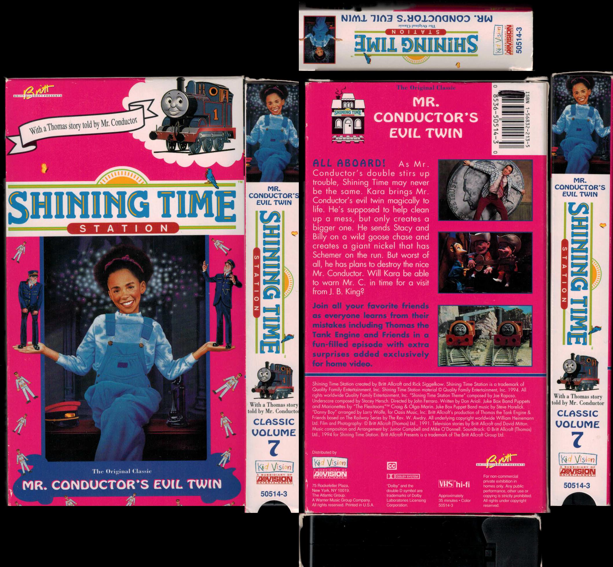
Many scanners have the ability to scan directly to PDF, and these frequently support multi-page PDFs. Thus, it doesn’t take much time to scan one side, flip the box, scan another, and so on until all the artwork has been saved. Figure 1 shows a the thumbnails of a sample PDF. The order I prefer for the six box sides is front-left-back-right-top-bottom; pdf2boxart is hardcoded to expect this order at present but could be adjusted with minimal effort.

Figure 1: Sample PDF showing a separate box side on each page

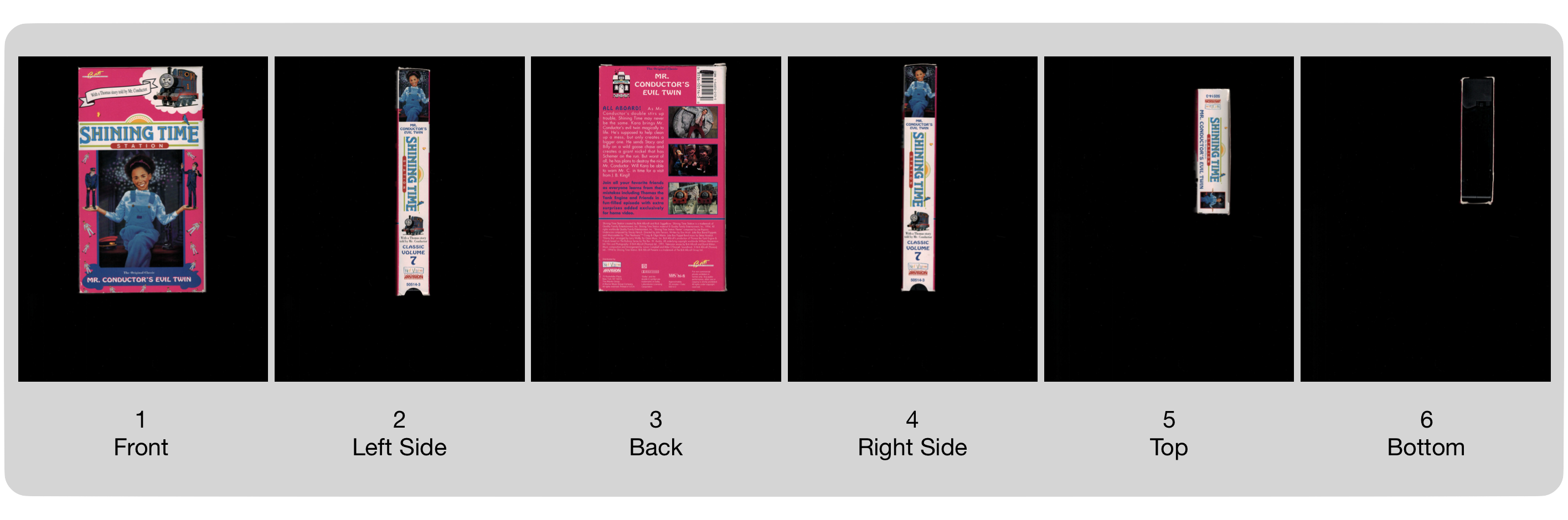
The example used in Figure 1 is a cover from the classic Shining Time Station TV series. This was a very well-done show that was both calming and entertaining to watch. It also brought Thomas the Tank Engine to television, helping to popularize the character as a children’s toy. Sadly, the series has never been released on DVD and so may be lost to time, apart from the few VHS releases that were made in the 1990’s.²

Once the PDF has been created, run the pdf2boxart script to begin processing:

./pdf2boxart.py input.pdf <optional: window size (see Step 2)> <optional: threshold (see Step 3)>

Step 2: Downsampling

When it starts, pdf2boxart will read the input PDF or directory of PDFs into a set of images using pdf2image:

images = pdf2image.convert_from_path(filename)

Then a couple of steps are combined during segmentation, but for the purposes of walking through this example, the steps have been split apart. We’ll start with downsampling since that decides the values upon which segmentation will operate.

Sliding Window

The window size parameter determines the number of pixels which will be considered when downsampling. For a window size of w, a “window” of wxw pixels will be “slid” across the image, computing the average pixel value within the window at each step. The act of sliding the window across the image is unsurprisingly called “sliding window”, and it is a very common algorithm for doing detection or segmentation within images. In this case, the window defaults to 26x26 pixels (randomly selected based on my testing a small number of images) with an overlap of 0, so the window moves 26 pixels each time.

A sliding window is easy to create in code. A nested loop allows the window to iteratively move along one dimension, and the outer loop increments the window in the other dimension at the end of each row. In the snippet below, the window moves along the x-axis to the right, computing a value at each step (an average in this case but could be anything), and then resetting to the start of the x-axis while incrementing along the y-axis.

# w is the window size defined by the user
i,j=0,0
while j + w < y: # Move along y-axis (down)
	while i + w < x: # Move along x-axis (right)
		avg = np.mean(img[j:j+w,i:i+w]) # Compute desired value
		i+=w # Step x
	i = 0 # Reset x at start of row
	j+=w # Step y

Figure 2: Animation of a sliding window

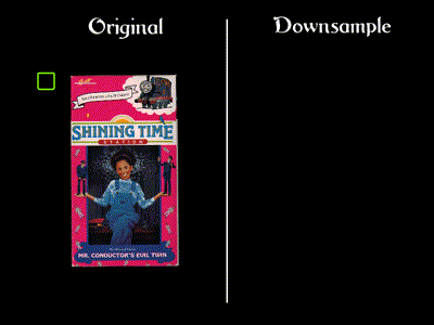
Figure 2 shows how the sliding window works with an animation of part of the process; the result is in Figure 3. Note that the scale has been exagerrated to better illustrate the process; the original image is much larger relative the window size that was used to generate the downsampled version here.

Figure 3: Result

As I mentioned above, the downsample is computed based on the average pixel value within each window. This is a common way of downsampling an image, although many other approaches may be used. This process is closely related to two-dimensional convolution, which is an image processing technique which may be used to blur, sharpen, detect edges, or extract other features out of portions of an image. The key difference between convolution and downsampling is that the former does not change the size of the resulting image as the latter does. Convolution retains a consistent size by moving the “window” across each individual pixel rather than calculating a single value over the whole set of pixels at once. Wikipedia has a nice convolution article which explains the signal processing aspects of the operation, while Song Ho Ahn has a very good illustration of 2D convolution.

Kernels

You’ll notice from Song Ho Ahn’s page that when performing convolutions, the “window” is also called a “kernel”. The kernel refers to the weights within the window, representing a discrete function with which the input is being convolved. The sliding window used by pdf2boxart can also be considered a kernel. It uses an averaging function, although different functions could be used. For instance, while an averaging kernel will give equal weight to all pixels, a Gaussian kernel emphasizes central pixels.

Figure 4: Two kernels, one based on averaging and the other a Gaussian function

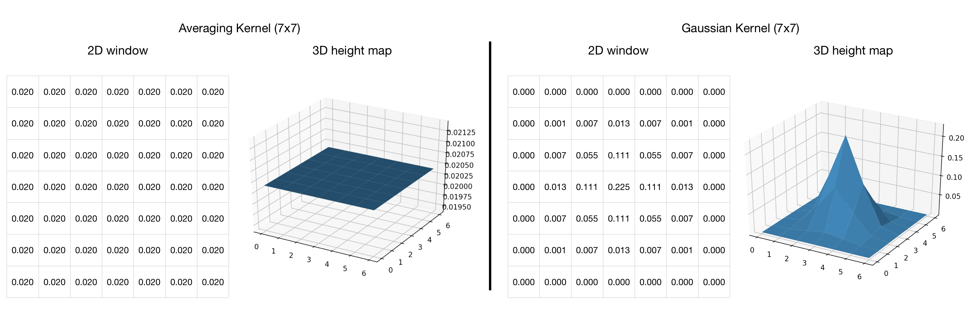
Figure 4 shows two 7x7 kernels. The left one gives equal weight to all pixels, AKA averaging. The general case for a window of size wxw is that each cell has the value 1/(w^2); in this example, each cell has 1/49 for the 7x7 window. The right kernel is a 7x7 Gaussian function. The weights of this kernel are more time-consuming to compute since a normal distribution of the desired mean and standard deviation must be generated. The values in this example were drawn from the sample kernel on Wikipedia’s Gaussian Blur page.

Figure 5: Comparison of the word "Conductor" from two kernels

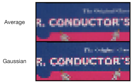
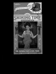
While a Gaussian kernel will blur an image through convolution, it can be used to create a sharper image when downsampling (recall that pdf2boxart is not performing an actual convolution, merely a similar sliding window process). Figure 5 illustrates the subtle difference between the two windows with downsampling. On the top is the result from pdf2boxart’s averaging process, and on the bottom is the result when a Gaussian kernel is used instead. The changes in pixel weight help sharpen certain attributes, particularly text as we see in the word “Conductor”.

Even though one kernel may result in sharper images than another, pdf2boxart uses the simpler averaging window because the downsampled image is not being saved anywhere. It only needs a temporary image to process with thresholding.

Step 3: Thresholding

In reality, pdf2boxart performs thresholding to identify edges for segmentation while sliding the averaging window across the image. For simplicity, let us assume the steps are done independently and that by this point, the program has a small, grayscale version of the input image like the one in Figure 3.³

Figure 6: A 2D image can be visualzed as 3D height map using the intensity of a pixel to set the height Figure 7: Panning to the top of the image to see the outline of the height map; tracing and smoothing shows how the row-level processing extracts edges

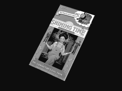
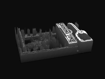
Image segmentation by thresholding is straightforward. First, the program determines a baseline value; pdf2boxart uses the upper left corner with the assumption that images will be more central on the page. Next, when averaging the pixels within each sliding window, the result is compared against the baseline. Lastly, if the difference between the average and the baseline exceeds the specified threshold, that window is marked as containing part of the image rather than background material. The next few subsections provide visuals for each step.

Intensities

All of the discussion to this point has referred to pixels, averages, and other computations as “values”, but a better term is “intensity”. The pixel intensity determines how “much” of a color to assign that pixel. Today, intensities are encoded as 8-bit binary values, one for each color channel.⁴ For grayscale, this means a pixel can have any value from 0 to 255, ranging from black (off) to white (on). In RGB, there will be a number from 0 to 255 for each channel of Red, Green, and Blue. The combinations of these channels yields the final color, allowing for millions of potentials – (2^8)^3 colors to be exact for 24-bit color (3, 8-bit channels).

A grayscale image is no more than a two-dimensional matrix of pixel intensities, and it can be easily visualized as a three-dimensional height map. Figure 6 illustrates exactly this process. As the camera pans by in a 3D space, the image is converted into a 3D surface. The height of any given point is based on the intensity, or lightness, of that pixel. Lighter portions become mountains while darker ones drop into troughs.

Row-level Processing

As the program computes average intensities with the sliding window, it is creating an array of averages across each row of the image. Building on our three-dimensional visualization from Figure 6, this is the equivalent of panning the camera around to the top of the image to where it rests upon the plane and then outlining the edges (intensities) along the face in front of the camera. Figures 7 illustrate both of these steps.

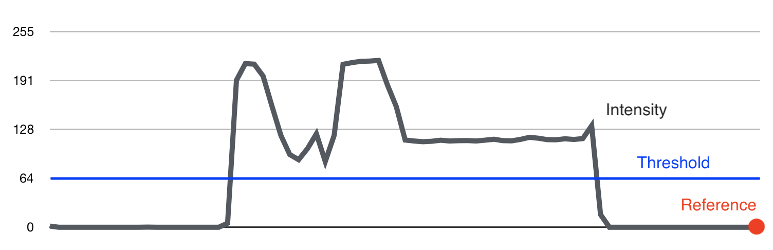
Comparison with Threshold

This line of pdf2boxart performs the actual thresholding:

out_thresh = abs(avg-ref_avg) > thresh # detect if this window average is outside thresh from reference

The user specifies the value of thresh, which determines how much the current window can deviate from the reference of the upper left corner. This method of segmentation relies on having a background that is mostly dark and solid. For a good scan, it is easy to see that the edges can be clearly detected.

Figure 8: The actual values from the example compare well with the approximation in Figure 7; any threshold below 128 would be sufficient for this example

Step 4: Box Art Spread

The final part of the workflow is to generate the full spread of box art. So far, the script has only relied on pdf2image for reading the images from the PDF and numpy to handle the matrix operations like averaging pixel intensities within a sliding window. To create the spread, PIL, the Python Image Library, is used. PIL aggregates a lot of useful image functions into an easy-to-use package.

Assuming the box sides were scanned in the order identified by Figure 1, pdf2boxart will step through each segmented image and concatenate onto the previous one. This answer on Stack Overflow provided the basis for the logic used in pdf2boxart to do the image joining.

A final remark worth noting is that the direction of the top and bottom scans are not important to pdf2boxart since it will rotate them to be placed above and below the back of the box.

Once all images have been processed and segmented, the final result is saved to a new file based on the input filename. Figure 9 shows the full spread based on the input of Figure 1.

Figure 9: Full box art spread